Okieinexile's Blog

By Bobby Neal Winters

Introduction

I have a series of exercises that I use in my Elementary Statistics classes which involve M&Ms Chocolate candy. They may be found at my Redneck Math blog which I have not used for a while. Over the past few weeks, I’ve been teaching my class in a compressed schedule in Paraguay.  In addition to this, in the Spring semester, I agreed to be on the committee of a student in my university’s Doctor of Nursing Practice Program.  In my spare time here in Paraguay–of which I have a lot–I’ve been investigating one of the statistical tests that this student is going to use: Fisher’s Exact Test.

The reader might very well be mystified by the name of the test.  I know that I was.  I had never heard of it before.  I am a mathematician, not a statistician. There is a difference.  Both the mathematicians and the statisticians are adamant on this point. I informed the DNP student of this.  She replied that she had every confidence in me.

Okay.

So I looked it up. As it turns out, her confidence was well placed.  Fisher’s Exact Test is a manifestation of the Hypergeometric Distribution.  This is a discrete probability distribution that I have been teaching in my Elementary Statistics Class years.  I do mean literally years. Decades in fact. Oh, God, I am aging even as I write this.

Let us continue.

Brief Explanation

In a nutshell, it calculates the probability of sampling without replacement.  Say you have a container of some sort, say a can, that contains the number $a$ of red beads and the number $b$ of blue beads.  Suppose that you’ve been blind folded, and you reach in and take a handful of the number $n$ of beads. What is the probability that you will have the number x of red beads in your hand? 

Oh, exciting stuff.

There is a formula for this and everything. I hope that you will not feel misused if I omit the particular formula at this time. For those of you who must know, I will give it to you near the very end of this article.  All you need to know right now is that we can calculate the probability that your handful of $n$ beads of any color will contain $x$ beads of the color red.

Of course there is nothing magic about the color red.  We could switch them around.  We don’t even have to have only two colors.  We simply need to have two groups that can be differentiated from each other. One group–the group we ask the probability question about–called success and the other, failure.

The M&M Experiment

For my M&M experiment, I brought a couple of packages of the “fun size” bags of M&Ms from the US.  These packages of are the type one would get in preparation for Halloween. To keep from saying packages of packages, we will say the packages contained bags of the M&Ms candy.

They do have M&Ms in Paraguay. Now.  That hasn’t always been the case, and I haven’t found the fun size bags yet. So, even though I only ever rose as high as cub scout and only held that rank for a year, I was prepared.

The first M&Ms assignment goes like this.  Take a fun size bag of M&Ms; count the red ones and write this number down; do this for the orange ones; for the yellow, the green, the blue, and the brown.  Do this for each package.  For this class, the students were able to have 22 packages.

What they see is this: Variation.  For each color, there is a different number in each bag.  Not every color appears in every pack.  This is the data the class took:

Bag ID	RED	ORANGE	YELLOW	GREEN	BLUE	BROWN
1	4	1	5	4	1	1
2	2	4	2	2	2	3
3	2	3	3	5	2	0
4	0	3	4	1	4	3
5	3	3	2	2	3	3
6	3	2	3	1	0	6
7	1	6	3	2	1	1
8	0	3	3	1	6	2
9	2	5	4	0	3	1
10	0	2	2	5	6	0
11	1	2	3	4	3	2
12	1	2	5	1	2	2
13	6	1	1	2	5	1
14	2	6	3	0	3	1
15	0	5	1	3	5	2
16	2	4	3	5	0	1
17	2	4	2	2	4	2
18	1	3	4	1	4	3
19	3	1	4	1	3	3
20	1	3	3	0	5	3
21	2	2	5	1	3	3
22	2	1	4	1	1	6

A Quick Glance at the Data

A quick glance at the data will show you that there is variation in color per bag.  If you stick it in a spreadsheet, you will note that there is a variation in the total number of M&Ms per bag just as there is with color.  In the case of the total number of M&Ms per bag, the variation is less.  The minimum number was 13 and the maximum number was 16 with frequency as given in the following table:

Number of M&Ms per Bag	Frequency
13	1
14	1
15	13
16	7

Note that, while there is variation, most of the bags contain 15 M&Ms total.  

A Thought Experiment

Consider now the following thought experiment.  We will be filling bags with M&Ms.  One might imagine that the various colors are each made separately, and then mixed in random fashion within a large bin.  There is then a process to fill each bag.  For the sake of simplicity in the math that follows we will assume that each bag contains 15. 

For the process of filling, we may imagine a hand reaching in and removing one M&M at a time at random and transferring it to a bag until 15 are transferred in total. This is the paradigm of sampling without replacement whence the hypergeometric experiment arises,

Spreadsheets

We are now approaching the point when we will need to do some calculation. For this, a spreadsheet like Excel or Google Sheets is needed. It is fortunate that their syntax is not dissimilar. For the sake of my obsessive mind, I will include the Excel formula for the calculation of hypergeometric probability. Healthier minds may feel free to skip the rest of this section. But don’t. It’s not hard.

The probability $P(X=x)$ for $x$ successes in a sample of $n$ may be calculated as

$P(X=x$) = HYPGEOM.DIST( x, n, a, a + b, FALSE)

where

• x is equal to the number of successes in the sample
• n is the size of the sample
• a is the number of successes in the population
• a + b is the size of the population, so therefore, b is the number of failures
• FALSE is there because we want this function to calculate only a single, not a cummulative, value

Seeing Red

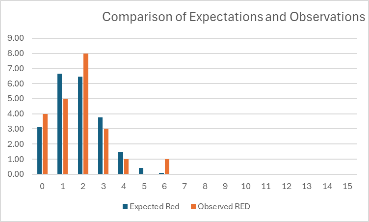
To me, red is the most easily distinguishable color of the M&Ms, so I use it as an example. In our data, we had 334 M&Ms total. Of these, 40 were red. Given this data, we can use our spreadsheet to calculate the probability that a bag of 15 M&Ms will contain 0 red M&MS is 0.14. (We write this as $P(X=0)=0.014$.) Given that we had a total of 22 bags, this means that we would expect (0.14)(22)= 3.11 of those 22 bags to contain no red M&Ms. We can do this calculation for number of red x=0, none of the M&Ms are red, up to x=15, all of the M&Ms are red, to get the following table:

x	P(X=x)	Expected Red	Observed RED
0	0.14	3.11	4
1	0.30	6.66	5
2	0.29	6.47	8
3	0.17	3.78	3
4	0.07	1.48	1
5	0.02	0.41	0
6	0.00	0.08	1
7	0.00	0.01	0
8	0.00	0.00	0
9	0.00	0.00	0
10	0.00	0.00	0
11	0.00	0.00	0
12	0.00	0.00	0
13	0.00	0.00	0
14	0.00	0.00	0
15	0.00	0.00	0

While glancing at these numbers might give you an idea that the expectations fit the observed reality quite well, the graph comparing the two is quite compelling:

The Assignment

After I walked the students through this, I gave them the group assignment to replicate it for each of the other colors. They could choose to work it all themselves–which some did–but they could also choose to divide it up, as was my intention.

Fisher’s Exact Test

I will confess that creating this assignment with my students was done in order to force myself to increase my knowledge for the sake of the doctoral committee I am on. That is to say, I want to understand Fisher’s Exact Test.

Fisher’s Exact Test is an example of a test of statistical significance. As a mathematician, it has taken me a while to fit these sorts of tests into my way of thinking. They are not determiners of truth or falsity. One way to think about them is means to justify actions. You might be right; might be wrong; but you have an idea of the probability of each of those and can gauge the cost of your action in the light of those probabilities.

The Basic Idea of a Test of Significance

To understand a test of significance in an intuitive way, imagine that your friend is a fisherman. He’s come back from a fishing trip having caught a fish. You ask him how big the fish was. If he holds his hands out and the tips of his fingers are only a few inches apart, then you believe him without question. However, if he holds his hands out and they are a few feet apart, then you call him on his exaggeration.

Somewhere, between those two extremes, you set a distance that claims of a fish larger than this size are not plausible.

In statistical tests of significance, we can associate a probability with that distance. This probability is called the significance of the test. The smaller the significance of a test, the less likely the chance that you are to call you friend a liar and be wrong.

Fisher’s Exact Test: The Details

In order to understand Fisher’s Exact test, let’s concentrate on a simple example. Let’s say we are trying to test the efficacy of a fertilizer on plants. The researcher has a study group of $N$ plants. Of those $N$ plants, $T$ are given the fertilizer and $U=N-T$ are kept as a control group. At the end of the study, some means has determined whether the treatment with the fertilizer has been successful or not. We will denote the number on which the treatment has been successful as $S$ and the ones on which it has not as $F = N-S$. We summarize this in the following table:

	Treated	Control
Successes	a	b
Failures	c	d

To summarize:

• T = a + c
• U = b + d
• S = a + b
• F = c + d

Now we look at the successes. The idea is to see whether the number of treated is so large within the test group as to be unlikely the work of simple chance. This is similar to the idea that we would reject our friends fish story if the size of the fish is too big. In this method, we arrange the question this way: Is the number of treated items among the successes so large that we doubt this is a matter of chance?

We now examine the set of successes within the study in order to determine whether items from the treated group are disproportionally represented. Suppose that there are $a$ successes. The the probability of getting $a$ or more successes can be calculated exactly is

One would imagine that the reason this is called Fisher’s Exact Test is that we can compute this probability $p$ exactly. It’s just there in the name. The smaller the value of $p$ the less likely this is to happen by chance. In most disciplines there will be an agreed threshold value for $p$ that will determine whether the result will be accepted by the discipline.

A key thing to remember is that unlikely things happen all the time. This should lead us to be humble, but, somehow, we aren’t.

An Example with Numbers

In order for us to get a better grasp of the process, let us work through this with some numbers I have pulled out of thin air for this very purpose. Let us assume the study group contains $N = 60$, and, of that number, $T = 30$ receive the treatment. This leaves $U = 30$ in the control group. Let us again suppose that after the study, there are $S = 20$ successes and that of those successes $a= 15$ had received the treatment so that $b=5$ of the successes were from the control group.

What is the probability that there would be 15 or more treated items among 20 items from our study group. We can calculate this with the aid of the table below, which was calculated using Google Sheets.

x	P(X=x)	P(x<=1)	P(X>=x)
0	0.00	0.00	1.00
1	0.00	0.00	1.00
2	0.00	0.00	1.00
3	0.00	0.00	1.00
4	0.00	0.00	1.00
5	0.01	0.01	1.00
6	0.02	0.03	0.99
7	0.06	0.09	0.97
8	0.12	0.21	0.91
9	0.19	0.39	0.79
10	0.22	0.61	0.61
11	0.19	0.79	0.39
12	0.12	0.91	0.21
13	0.06	0.97	0.09
14	0.02	0.99	0.03
15	0.01	1.00	0.01
16	0.00	1.00	0.00
17	0.00	1.00	0.00
18	0.00	1.00	0.00
19	0.00	1.00	0.00
20	0.00	1.00	0.00

The first column is the number of treated among the successful. The second column is the probability of that occurrence. The third is the cumulative less than or equal to that number, and the last column is the probability of that number or more. Technically, you only need to see the first and last columns, but I did the work, so there it all is.

Note that for this example $p = 0.01$ so this is only likely to happen one percent of the time. Impressive, but then I made it up.

The Formulas

Okay, I’ve put this off until now in order to avoid scaring people with the hypergeometric probability formula. For the people I teach it to–nonmathematical general education students–it is likely the scariest formula they have ever seen. Letting $X$ be the random variable that counts the number of successes from $n$ trials from a population that had $a$ successes and $b$ failures:

Here the notation $\binom{n}{r}$is the so-called binomial coefficient. It is the number of subsets with $r$ elements that a set of $n$ elements have. If you are lucky–and most of my students are–you have a button on your calculator for this that is often denoted as $_nC_r$. If you are not so lucky, then you can calculate it by the formula

The $()!$ notation is referred to as “factorial.” You probably have calculator key for it. If not:

We learn this in small bites, like eating an elephant, but the somewhat tortured syntax in Excel isn’t looking so bad now, is it?

Acknowledgements

I would like to thank my students over the years for helping me think this all out. In particular, I would like to thank the students Renato, Maria, Kathia, Constanza, Victoria, and Abigail who were in the group that collected the M&Ms data for their help.